C is for Cycle Time [Part 1]

This two-part article aims to explain how we can improve cycle time in front-end semiconductor manufacturing through innovative solutions, moving beyond conventional lean manufacturing approaches. In part 1, we will discuss the importance of cycle time for semiconductor manufacturers and introduce the operating curve to relate cycle time to factory utilization. Part 2 will then explore strategies to enhance cycle time through advanced scheduling solutions, contrasting them with traditional methods.

Part 1 

Why manufacturers care about cycle time 

Cycle time, the time to complete and ship products, is crucial for manufacturers. James P. Ignazio, in Optimizing Factory Performance, noted that top-tier manufacturers like Ford and Toyota have historically pursued the same goal to outpace competitors: speed ^[1]. This speed is achieved through fast factory cycle times.

This emphasis on speed had tangible benefits: Ford, for instance, could afford to pay workers double the average wage while dominating the automotive market. The Arsenal of Venice's accelerated ship assembly secured its status as a dominant city-state. Similarly, fast factory cycle times were central to Toyota’s successful lean manufacturing approach.

Furthermore, semiconductor manufacturers grapple with extended cycle times that can often span 24 weeks ^[2]. This article will focus on manufacturing processes in front-end wafer fabs as their contribution to the end product, such as a chip or hard drive disk head, spans several months. In contrast, back-end processes can be completed in a matter of weeks ^[3]. However, the principles discussed apply universally to back-end fabs without sacrificing generality.

Why Short Cycle Times Matter for Front-end Wafer Fabs

• Revenue acceleration: The quicker products reach customers, the faster revenue streams in. However, quantifying the precise financial impact due to cycle time is intricate and beyond this article's scope.

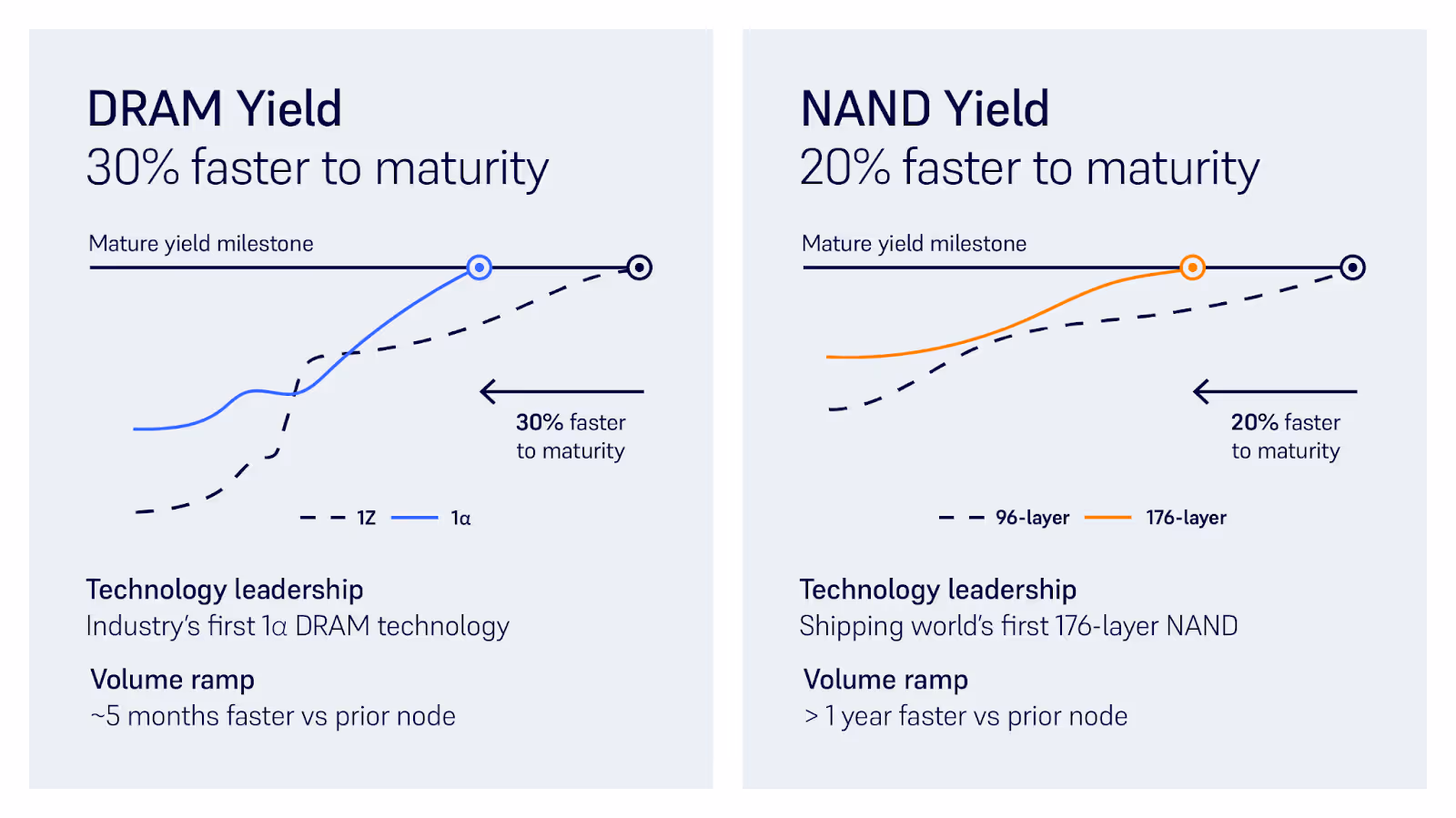
• Competitive advantage: Gaining a competitive advantage involves reducing cycle time in R&D wafers, which accelerates product launches. More than 20% of front-end fab production lines can be used for R&D wafer testing and iteration. Swift deliveries enhance a company's reputation, leading to more contracts. At the 2022 Winter Simulation Conference, Micron highlighted their rapid advancements: maturing 30% quicker in DRAM (five months ahead of the previous node) and 20% in NAND (a year faster than the prior node). See Figure 1.

• Agility in market responsiveness: A fab with shorter cycle times can swiftly adjust to market fluctuations, whether that is a surge in demand or a shift in product preferences, such as changes in product mix. It can also respond faster to changes in customer requirements.

• Risk mitigation: The shorter the cycle time, the quicker a fab can respond once defects have been detected as it takes less time to perform rework.

• Inventory management: Lower cycle times can reduce the amount of work-in-progress (WIP) in buffers or racks (intermediate stock), or stock at the end of the production line. This not only liberates tied-up capital but also wafers can move quicker with less WIP in the fab as it is shown in a later section introducing the operating curve.
  ‍

Achieving Predictable Cycle Time

Less variability in cycle time helps a wafer fab to achieve better predictability in the manufacturing process. Predictability enables optimal resource allocation; for instance, operators can be positioned at fab toolsets (known as workstations) based on anticipated workload from cycle time predictions. Recognizing idle periods of tools allows for improved maintenance scheduling which will result in reduction in unplanned maintenance. In an upcoming article (Part 2), we'll explore how synchronizing maintenance with production can further shorten cycle times.

Measuring and monitoring the cycle time improves overall fab performance

Measuring and monitoring cycle times aids in identifying deviations from an expected variability. This, in turn, promptly highlights underlying operational issues, facilitating quicker issue resolution. Additionally, it assists industrial engineers in pinpointing bottlenecks, enabling a focused analysis of root causes and prompt corrective actions.

Supply chain stakeholders usually fail to understand the impact of cycle time 

In the semiconductor industry, cycle time plays a pivotal role in broader supply chain orchestration:

• A predictable cycle time informs suppliers when to provide fresh batches of raw materials. 
• Furthermore, it influences the downstream processes of Assembly & Test Operations (back-end facilities). Back-end facilities with a cycle time of less than a week gain enhanced predictability, allowing for more effective allocation of capacity and resources.
• Predictable cycle times will also inform safety inventory levels, freeing capital and optimizing storage space. 
  ‍

Cycle time is a component of the total lead time of a product (it also includes procurement, transportation, etc). Therefore, total lead time can be reduced if the long cycle times in the front-end wafer fabs are reduced. A reliable cycle time nurtures trust with suppliers, laying the foundation for favorable partnerships and agreements. In essence, cycle time is not just about production; it's the heartbeat of the semiconductor supply chain ecosystem.

Understanding how cycle time impacts product delivery times is essential for the semiconductor industry. In some analyses, you could see that cycle time is confused with capacity, as the authors in a McKinsey article stated “Even with fabs operating at full capacity, they have not been able to meet demand, resulting in product lead times of six months or longer” ^[4]. On the contrary, in a fab operating at full capacity, lead times of the products will increase as the average cycle time of manufacturing is increasing. 

How to measure cycle time

Fab Cycle Time

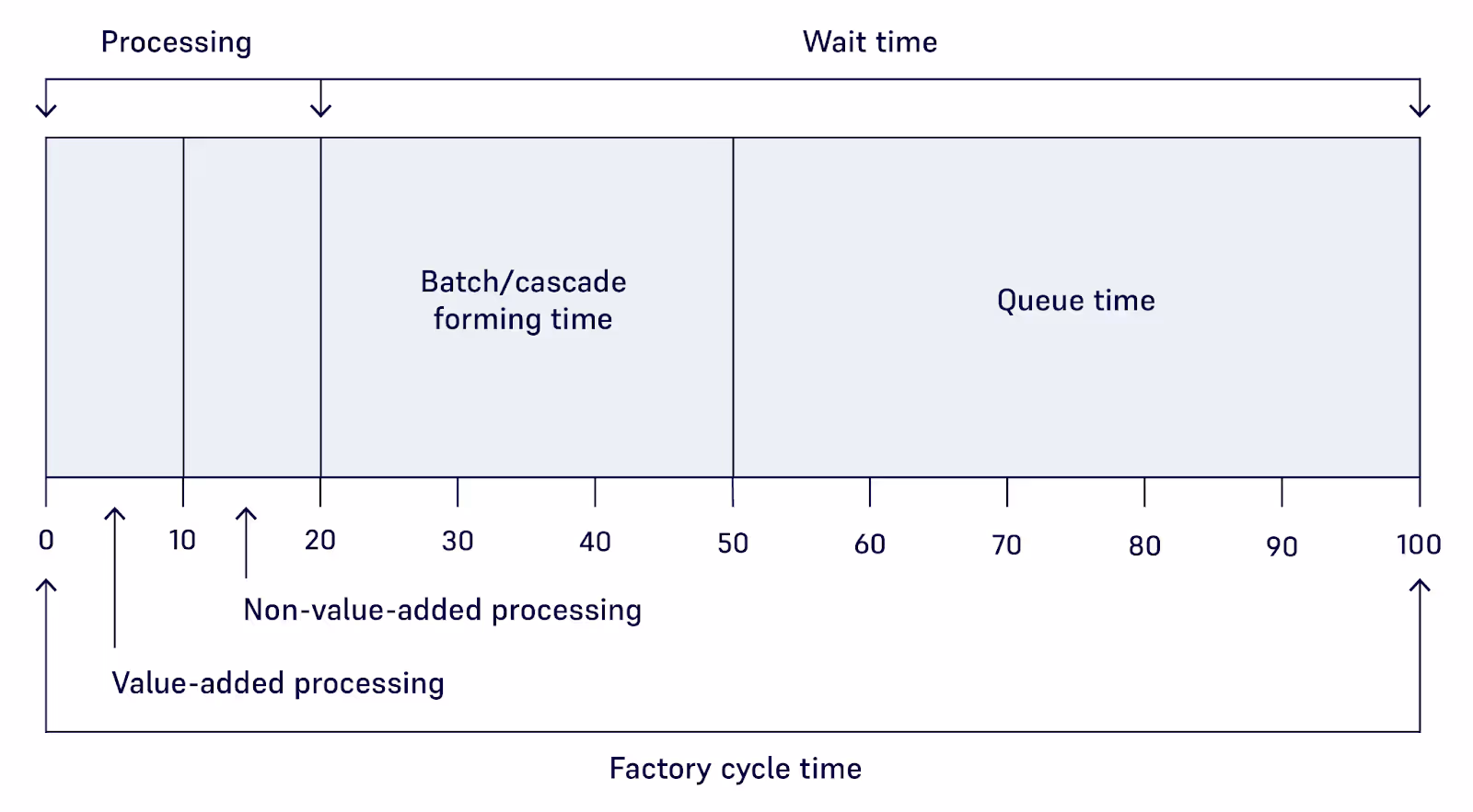
The fab cycle time metric defines the time required to produce a finished product in a wafer fab. The general cycle time term is also used to measure the time required to complete a specific process step (e.g. etching, coating) in a toolset, known as process step cycle time. The fab cycle time consists of the following time components as can be seen in Figure 2:

• Value-added processing time, which is the time taken to transform or assemble the unfinished product, which is a wafer in our case.

• Non-value-added processing time includes the time taken for inspection and testing, as well as the time for transferring the wafer between different steps.

• Time to prepare the products for processing: this refers to the time operators or tools required to form a batch, i.e. to select which lots should be bundled together for processing.

• Queue time: the time spent where the unfinished wafer is waiting to be processed because the tool required is busy, due to the tool processing another batch or undergoing maintenance.
  ‍

To measure and monitor cycle time, wafer fabs must track transactional data for each lot, capturing timestamps for events like the beginning and completion of processing at a tool. This data is gathered and stored by a Manufacturing Execution System (MES). Such transactional information can be utilized for historical operations analysis or for constructing models to forecast cycle times influenced by different operational factors. This foundation is crucial for formulating the operational curve of the fab, which we'll delve into in the subsequent part of this blog. As outlined in an article by Deenen et al., there are methods to develop data-driven simulations that accurately predict future cycle times ^[3].

Fab operating curve: Fab Cycle Time versus Factory Utilization

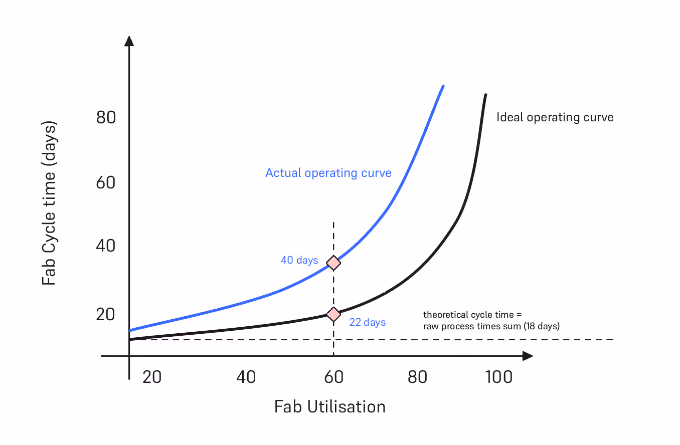
As we mentioned earlier, historic data can be used to generate the operating curve of a fab which describes the cycle time in relation to the factory utilization. Figure 3 shows the graph of the fab cycle time in days versus the utilization of the fab (%). The utilization of the fab is defined as the WIP divided by the total capacity of the fab. 

We have found this method useful in understanding the fundamental principles of cycle time. The operating curve helps to explain how factory physics impact fab KPIs such as cycle time and fab utilization by showing the changes in the operating points: 

• The horizontal line, representing the summation of raw process times (known as theoretical cycle time), envisions a scenario with zero queuing time in the fab. This illustrates the impact of queuing time on cycle time as we increase WIP, moving right on the x-axis. Accumulation of queuing time becomes inevitable with the introduction of more WIP in the fab.
  ‍
• The ideal operating curve represents the operation of a wafer-fab assuming that there is zero waste. This curve defines the minimum achievable cycle time for each fab load and the difference between this curve and theoretical cycle time is because of real life variability in the fab that cannot be eliminated completely, e.g. unplanned maintenances, inconsistent tool processing times.
  ‍
• The cycle time tends to go to infinity, when you move towards 100% utilization of the fab.
  ‍
• The actual operating curve, cycle time versus factory utilization, represents the current fab’s operation considering all the inefficiencies such as excessive inventory, variability in operations, idle times, poor batching and rework.
  ‍
• Both curves assume average or constant values of the operational parameters of the fab for example a fixed number of tools installed, an average availability of each tool and labor, and a constant product mix.
  ‍
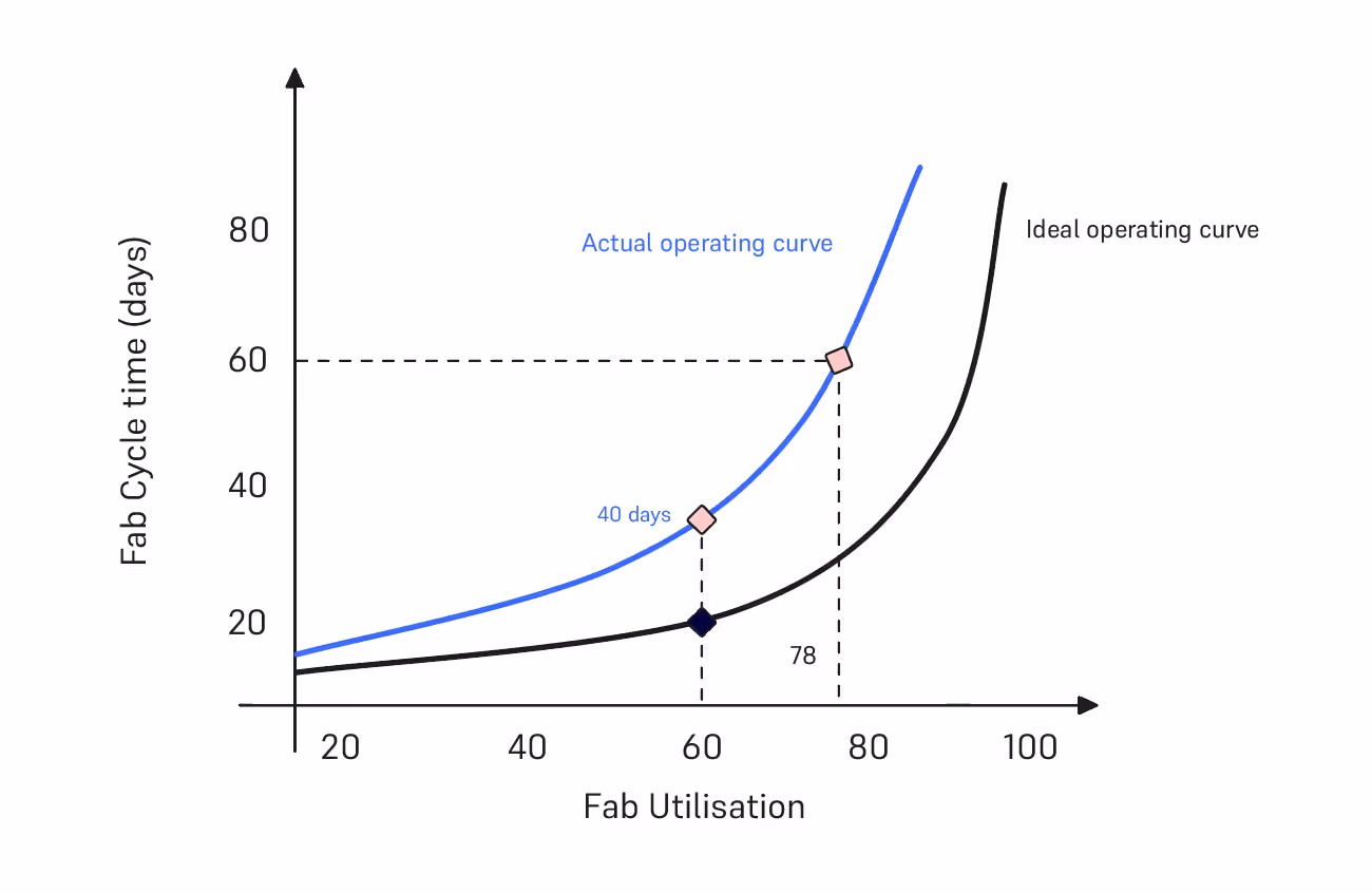
• The actual operating curve describes the impact on cycle time if we load the fab with more WIP as shown in Figure 4. The fab management could use this information to make a decision about the trade-off between cycle time and factory utilization. Higher fab utilization is associated with a higher throughput (i.e. number of wafers per unit of time).

In Figure 3, you can see that the current fab cycle time is 40 days when the factory utilization is at 60%. Theoretically, we could reduce the cycle time to 22 days. The difference between these two points is due to the inefficiencies that contribute to the factory cycle time as explained in the introduction of this section. In Part 2 of this blog, we will explore the various types of inefficiencies and examine how innovation can shift the operating curve to achieve lower cycle times while maintaining the same fab utilization.

Summary 

In summary, cycle time is not merely a production metric but the very pulse of the semiconductor manufacturing and supply chain. It governs revenues, shapes market responsiveness, and is pivotal in driving innovation. By understanding its nuances, semiconductor companies can not only optimize their operations but also gain a competitive edge. And while we've scratched the surface on its significance, the question remains: how can we further reduce and refine it? In part 2 of the C for Cycle Time blog, we will discover innovative techniques that promise to revolutionize cycle time management in wafer fabs.

‍

Author: Dennis Xenos, CTO and Cofounder, Flexciton

References

• [1] James P. Ignizio, 2009 ,Optimizing Factory Performance: Cost-Effective Ways to Achieve Significant and Sustainable Improvement 1st Edition, McGraw-Hill, ISBN 978-0-07-163285-0
• [2] Semiconductor Industry Association, 2021, Blog, URL
• [3] Deenen, P.C., Middelhuis, J., Akcay, A. et al., 2023, Data-driven aggregate modeling of a semiconductor wafer fab to predict WIP levels and cycle time distributions. Flex Serv Manuf J. https://doi.org/10.1007/s10696-023-09501-1
• [4] Ondrej Burkacky, Marc de Jong, and Julia Dragon, 2022, Strategies to lead in the semiconductor world, McKinsey Article, URL. 

‍