Multi-objective Fab Scheduling: Exploring Scenarios and Tradeoffs for Better Decision Making

Building and maintaining any form of scheduling solution to be flexible yet robust is not an easy undertaking. Commonly, fab managers have resorted to rule-based dispatch systems or other discrete-event simulation software to estimate how their fab will play out in the near future. Often this requires deciding a specific KPI that is important to the fab up-front; do I care more about getting wafers out the door, or reducing the cycle time of those wafers?

Competing objectives challenge

As a fab manager, there are a number of competing objectives to balance on the shop floor that all impact the profitability of the fab. Whether that be reliably delivering to customers their contractual quantities on time, or ensuring that fab research and development iteration time is kept low, fabs need a flexible, configurable scheduling solution that can produce a variety of schedules which account for these tradeoffs. At Flexciton, we call this “multi-objective” scheduling; optimizing the factory plan whilst considering several independent KPIs that, in this case, are fundamentally at odds with one another. This article explores Flexciton’s approach to multi-objective scheduling and how we expose simple configurations to the fab manager, whilst allowing our scheduling engine to ultimately decide on how that configuration plays out in the fab.

If there is no automated real-time dispatch system in the fab, determining the "best" schedule is a very complex procedure that cannot even be accomplished with advanced spreadsheet models. Assuming that the fab is advanced enough such that a dispatch system is in place, it will likely only consider "local" decisions pertaining to the lots that are immediately available to the dispatch system at the time the decision is made.

Dispatch systems typically do not have the configurability to adjust the user's incremental utility with respect to throughput and cycle time; they typically adhere to a series or hierarchy of rules that are tuned to consider exactly one KPI. Therefore to change the objective of the dispatch system would require rewriting these rules; an often time-consuming exercise that requires advanced technical knowledge of the dispatch system. This makes it almost impossible or otherwise very time consuming to trial various configurations of the fab manager’s preferences.

Balancing various objectives for best results

The Flexciton optimization engine is a multi-objective solution that can linearly balance various KPIs according to user-chosen weights. As these weights are exposed to the end-user, this renders the possibility of running many different scenarios with varying preferences trivial. Fab managers can have access to the specific weight values themselves or work with our expert optimization engineers to select from a handful of high-level configurations and the solution will select appropriate weights itself.

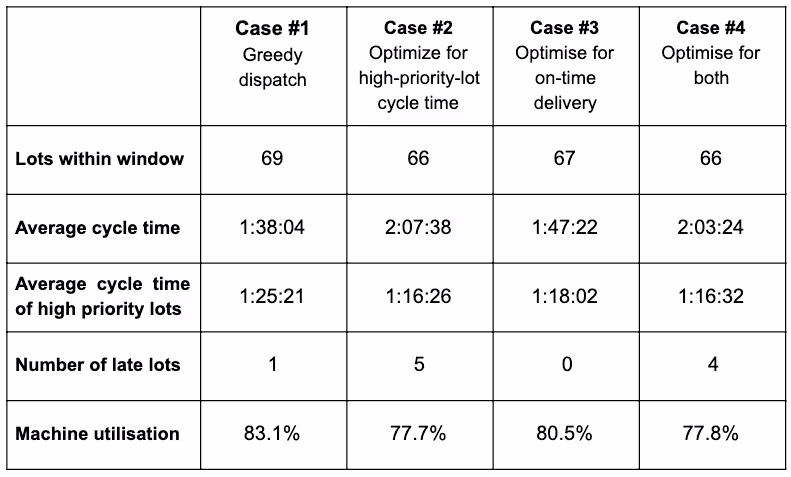
To properly understand the flexibility of the engine, we will now step through four case studies. The goal is to compare how, given the same dataset, slightly different objective configurations impact the solution that is returned by accounting for the change in preferences.

We present a schedule of nine tools from across five toolsets with seventy lots of a mix of 65% Priority1 lots. Each lot can go to a random subset of tools within a single toolset.

The schedule will then be tested against four runs:

1. Produced by a dispatch system with heuristic rules
2. Optimized for cycle time
3. Optimized for the on-time delivery of wafers
4. Balanced optimization considering both cycle time and OTD
   ‍

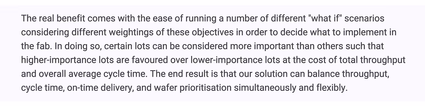
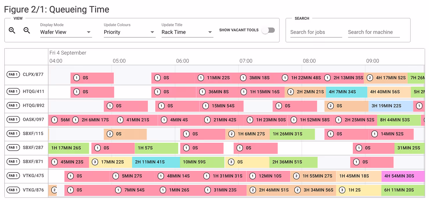
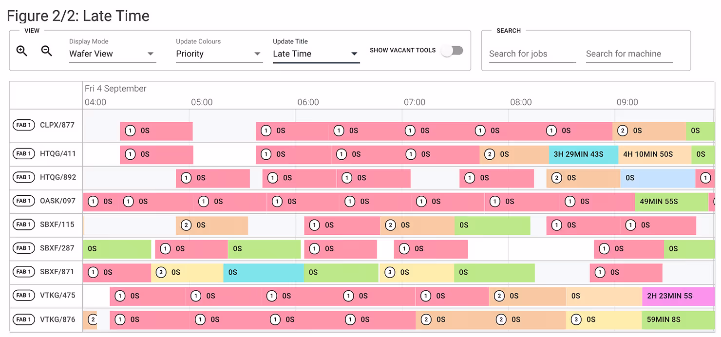
For each of these scenarios, we will present two gantt charts; one labelled with the “Queueing Time” of each lot (aka “rack time”) and another labelled with the “Late Time” of each lot. Late time refers to the duration by which the lot completed processing after its due date. If it was not late, the label reads “0s” since we do not consider being more early as being more favourable. Lots that are considered high priority (Priority 1 to 3) are given a circle badge indicating such. Low priority lots are Priority 4 through 10. Each lot is coloured according to this priority class.

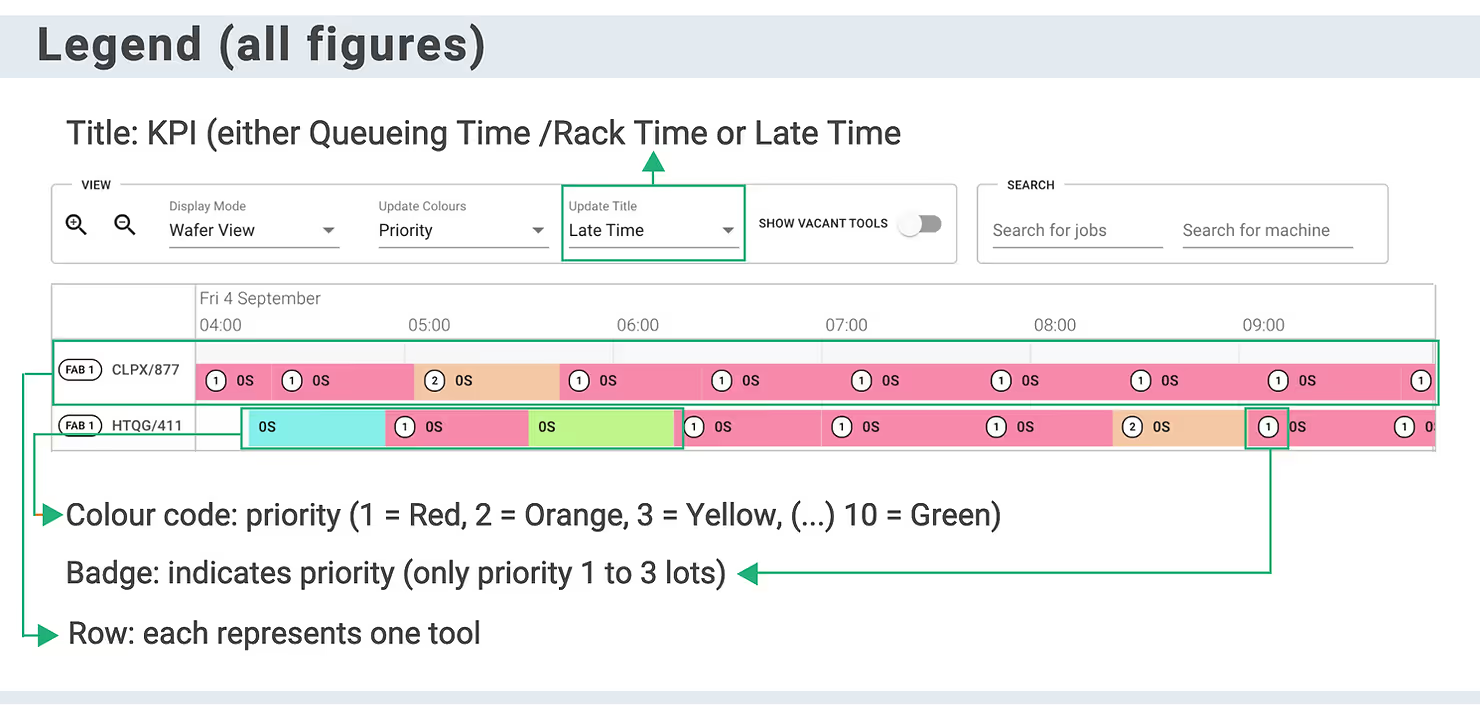
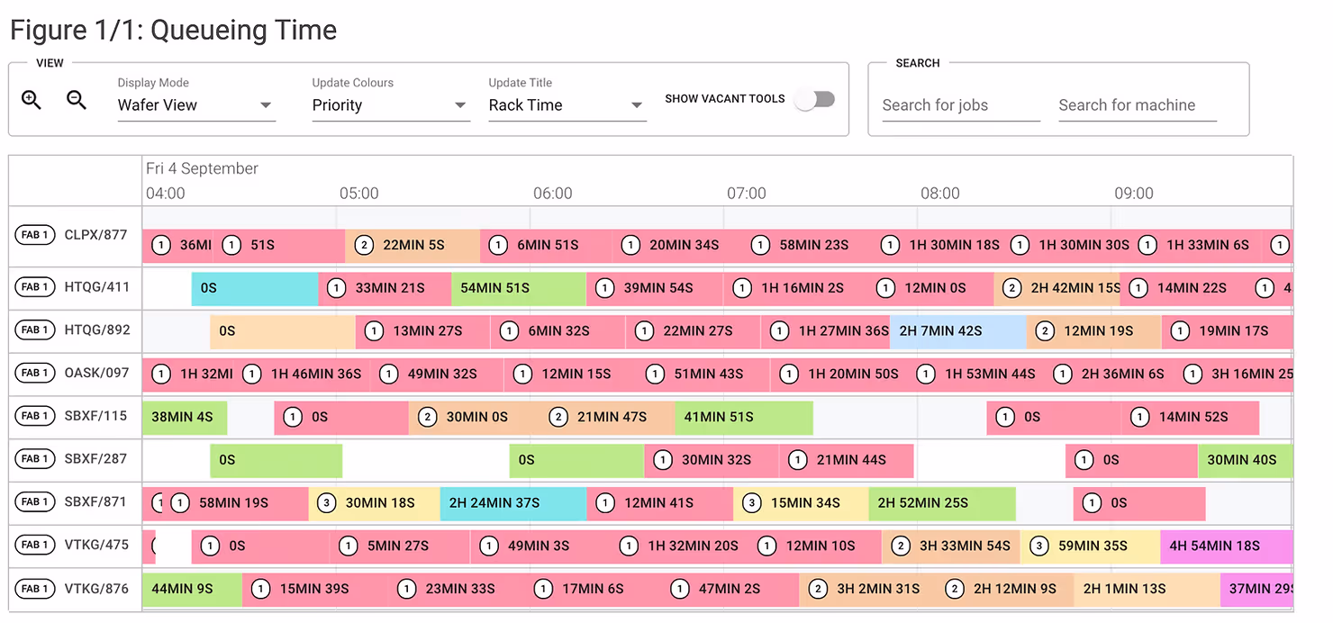
Case study #1: base case - greedy dispatch

To begin, we’ll present how a schedule could look when produced by a dispatch heuristic that does not consider the future arrivals of wafers, but simply what is currently available in front of a tool. The greedy rule here is to just dispatch the highest priority wafer on the rack at the point the tool is idle.

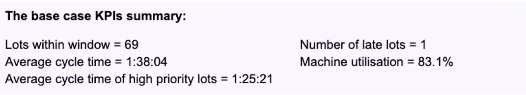
In the above example, the high-priority wafers have to wait due to the system only considering what’s on the rack and therefore dispatching the low-priority wafers that are ready to go.

It should be noted that such a strategy is great for improving overall throughput and cycle time since the machine idle time is reduced by constantly dispatching wafers. This has the side effect of delivering all-bar-one of the wafers on time. In reality though, not all lots are equal and fab managers care a great deal more about certain high-priority lots thus making the scheduling problem quite a bit trickier.

Unfortunately, in order to reconfigure the system to place greater importance upon the high-priority wafers and dispatch them first would require complex rewriting of the dispatch  rules to “look ahead” at the wafers that are not yet on the rack, and are arriving shortly. The dispatcher would then elect to keep the machine idle in order to reduce the high-priority wafer cycle time.

Case study #2: Optimize for high-priority-lot cycle time

Instead of modifying the RTD rules, we can emulate what that would look like by running our optimization engine whilst optimizing for the cycle time of high-priority lots:

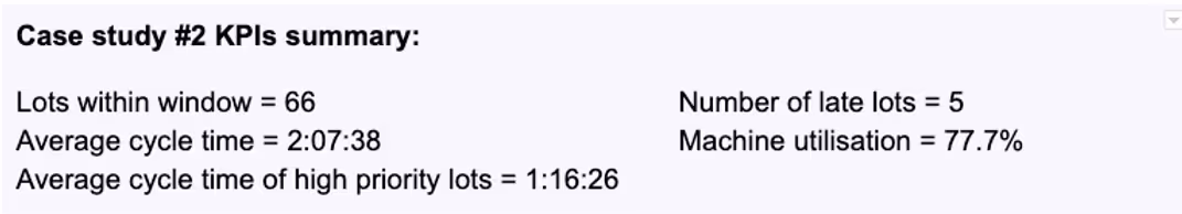
The low priority lots at the front of the schedule are replaced with high-priority lots so that they can be dispatched as soon as they arrive. These low priority lots have been pushed to the back of the schedule with non-zero rack time (since the cycle time of high priority lots matters so much more). Naturally this is at the cost of overall average cycle time which has suffered by 23% in order to improve Priority1 cycle time by 11%. Also note that on tool “SBXF/115”, our scheduling solution has pushed the Priority2 (orange) and the Priority10 (green) lots later so that the Priority1 (red) lots are rushed through with zero rack time.

Case study #3: Optimize for on-time delivery

With optimisation, there are no additional changes required to increase the flexibility of the system. We simply describe what a good schedule looks like using the multi-objective function and the optimizer does the rest. Subtle tweaks to this function will inevitably produce very different schedules. Now let’s take a look at how the schedule alters when we want to maximise solely on-time delivery.

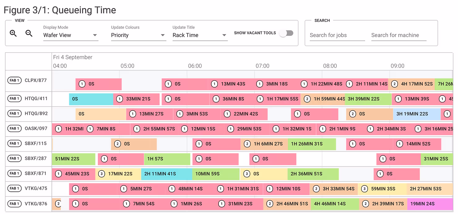
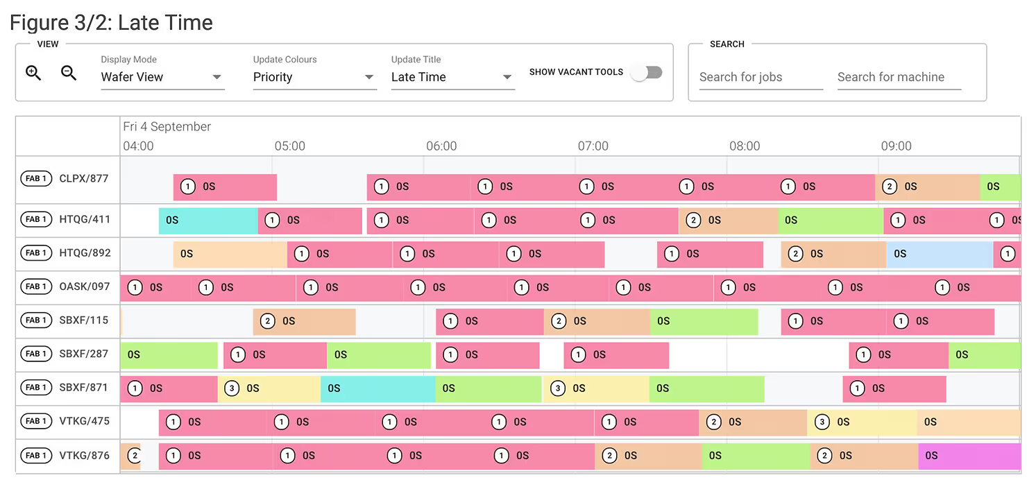
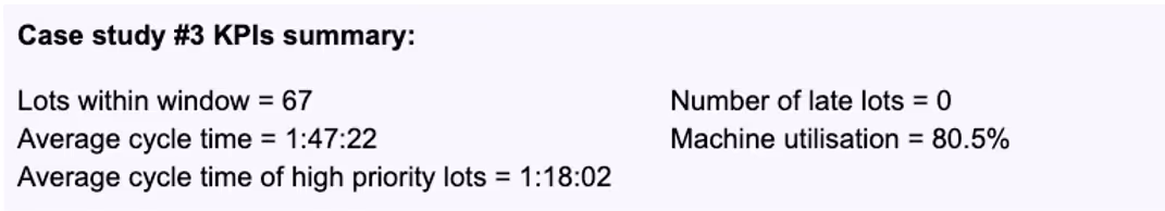
As expected, cycle time is quite a bit worse than previously however now there are no lots delivered late. This is very similar to the original schedule produced by simple dispatch rules. The low-priority lots have been brought forward so that they are delivered on time and the cycle time of the high-priority lots suffer as a result.

Case study #4: Optimize for both

Finally, the main purpose of this article is to illustrate the ease of considering both KPIs with some relative weight simultaneously.

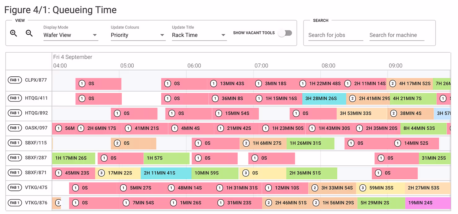
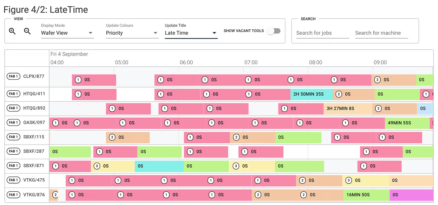
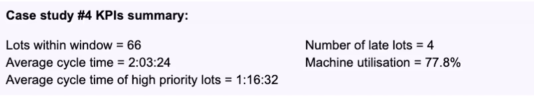
Note that the KPIs of cycle time and throughput are slightly worse than when that was the sole KPI being optimised. The key is that both are better than when the other KPI was being optimized. This balance is entirely in the hands of the fab manager. We maintain roughly the same cycle time of high-priority lots as when optimising for cycle time and fewer lots are late than when optimizing only cycle time.

Summary and Conclusions

This article has provided a number of ways that illustrate how optimization can be considered both more flexible and robust than heuristics that cannot effectively search the global solution space.

The engine is simple to tune due to the exposed weights and/or configurations presented to the fab manager which allow a high degree of customisation both with respect to the objective function and wafer priorities. This flexibility allows us to easily consider complex hierarchical objectives found in semiconductor manufacturing such as “optimise high-priority cycle time as long as no P1-8 lots are late” or “optimise batching efficiency (perhaps due to operator constraints) and then high-priority cycle time”. Ultimately, our solution is a market-leading scheduler that will realise true KPI improvements on your live wafer fabrication data.

Flexciton is currently offering the Fab Scheduling Audit free of charge. To enquire, please click here.

‍