To Batch or Not to Batch?

Batch tools are purposefully built to process two or more lots in parallel. However, due to the complexity and volatility of the wafer fabrication environment, each day, wafer fabs are challenged to make complicated batching decisions. How to determine when to batch lots together and when better not? This is what we shall call the ‘batch or not to batch dilemma’.   

Why batch lots together in a wafer fab?

One of the most precious commodities is time, and batch tools are designed to make the best use out of time. Often, these tools have a long processing time. An example would be a diffusion furnace. Instead of waiting for 6 or 8 hours for a single lot to go through the whole process before loading the next one, batching allows the processing of multiple lots simultaneously. This sounds like an easy way to solve a complex problem. However, with batch tools, on top of a whole host of constraints to respect, there are exponentially more scheduling options available compared to a non-batch tool.

In addition, the processing times of batch tools introduce a very complex dynamic. Batch tool processing times consist of fixed time (regardless of the number of lots in a batch) and a variable time (increases with each additional lot). Because of the fixed time component (+ tool setup time) in creating a batch, there is the perception that larger batch sizes are more efficient.

A typical approach to batching decisions

At a batch tool, there are a number of decisions to be made, such as whether you process lots that are already in front of the tool or wait for more to arrive? Additionally, if the number of lots waiting exceeds the tool capacity, which lots should you batch together and process first?  

Typically, each fab decides on their batch-size policy, which will guide the batching decisions. One of the commonly used policies would be a Minimum Batch Size (MBS) policy, setting a minimum number of lots required to start processing. This could be determined by running a large number of different simulations. These simulations will determine the batch size that provides the best performance for that specific use case. Thus, an MBS heuristic rule would be created, setting a certain direction to follow for all future lots.

On the other hand, a ‘near-full’ policy would require you to wait until the batch size is as close as possible to the maximum capacity of a tool. In this case, it is possible to achieve high throughput, but it can also cause the tool to stay idle for a long time when waiting for more lots to arrive in order to satisfy the policy, which negatively impacts on overall cycle time.

Processing a batch whenever the tool is available and ready to process, is another approach (this is called the ‘greedy policy’). This may reduce cycle time during times of low WIP, but will likely cause an increase to cycle time and lower throughput during times of high WIP.

How to determine the right batch size

The fact of the matter is that there isn’t one perfect batch size. In reality, it depends on the context of the whole system at that specific point in time. The batching decision relies on a number of dynamic factors:

• Max batch size constraints
• What will arrive and when
• What is currently in the queue
• Possible recipe combinations that can be batched together
• What priorities the wafers have
• What objective you are currently optimizing for
  
  ‍

In many fabs, daily batching decisions are guided by a dispatch system which uses rules-based heuristic algorithms. This approach can work very well in some cases but can bring very poor results in others.

Let’s take a look at an example, where we use a simplistic approach to illustrate the problem.

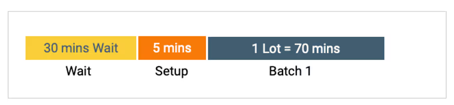
Suppose we have a batch tool with a maximum batch size of 4 lots. In order to get better efficiency, a typical dispatch rule is to set a minimum batch size e.g. minimum batch size of 2 lots. However, in a situation where one lot is already present, waiting too long, will be inefficient. Therefore, a maximum wait time - let’s say 30 min - would apply to the rule of minimum batch size. If we have waited 30 min, and another lot did not arrive, the dispatch system would send one lot for processing.

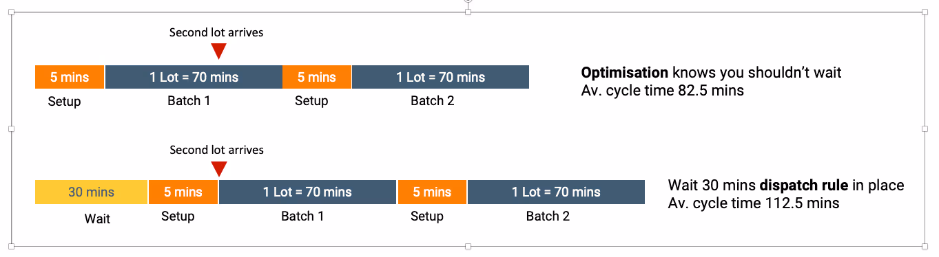
Sometimes this works well - here another lot arrived within 5 minutes, allowing  2 lots to be processed simultaneously.

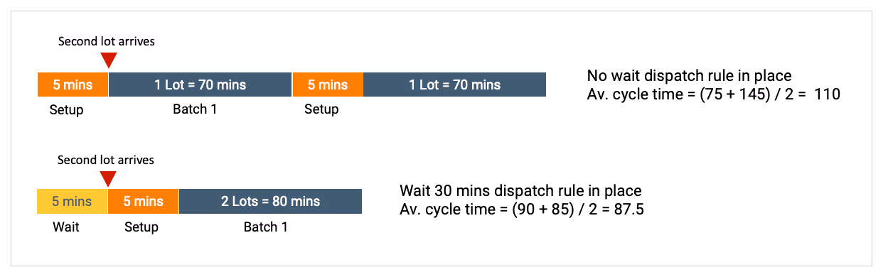
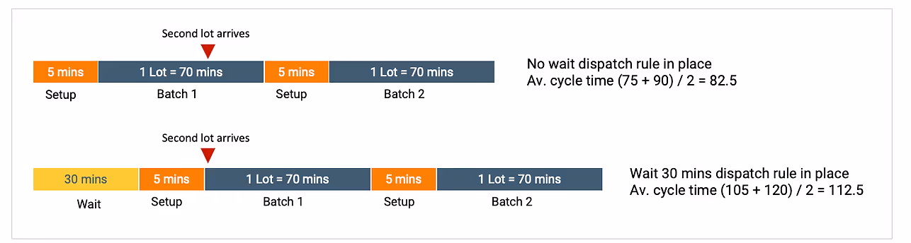
In this example, the rule was effective and achieved a lower average cycle time than if we hadn’t waited for the second lot to arrive. However, sometimes a rules-based dispatch system can make poor decisions. Typically the dispatch system will only make local decisions, and won’t look ahead to anticipate which lots and when are coming, as it’s illustrated in the second scenario below. The second lot arrives at the tool in 60 minutes, but due to the 30 min waiting rule, the first lot has already been dispatched.

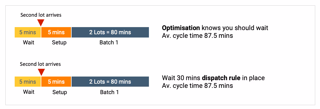
In order to make more optimal decisions around batch sizes, we need to be able to anticipate what WIP will arrive, when it will arrive, and where this WIP goes next after the current batching step.  This can be achieved by applying a smart scheduling approach which understands the broader context required to make optimized batching decisions. The below example illustrates a rules-based decision vs an optimization approach.

This is one very simple example which shows some of the trade-offs that must be considered when making batch decisions. In the above case, it would be possible to write an extension to the dispatch rules to account for the scenario presented. However, in reality, there are several other factors which bring additional complications. For example, often, Lots will have different priorities. When a high priority lot is batched together with a lower priority lot, the average cycle time for both lots may be reduced compared to running the Lots in two sequential batches. That said, the cycle time of the high priority lot is likely to be increased - this may be undesirable.

Given how dynamic a fab is, writing dispatch rules to efficiently deal with the full range of scenarios is possible, but would be extremely time-consuming to maintain and expensive to build.

Conclusion

Batch tools are extremely complex machines to schedule, as there is a huge number of scheduling options, and each option has a different efficiency. Commonly used dispatch rules can cause poor performance in a dynamic fab environment. Often, the batching methodology follows a fixed rule, such as maximum batch size. These fixed rules can provide occasional good outcomes, but they are unable to consistently provide good solutions. As a result, the KPIs across the batch toolset might show undesirable increases in cycle time, or reductions in throughput if the WIP mix or objectives change. Additionally, creating very efficient rules would require a lot of time and extensive maintenance.

Smart scheduling, on the other hand, introduces the ability to make optimized batching decisions in any situation to achieve the objective of increased throughout or lower cycle times. By applying mathematical hybrid-optimization techniques, we are able to find a solution which is near-global-optimal, delivering a consistently high-quality outcome.

Get your Wafer Fab Scheduling Performance Analysis fully remotely and free of charge. Click here to get in touch.

‍